Python Tutorial
This tutorial is meant to show you how to work with the symd. This will not focus on running simulations – see the other examples (symd) for that. Some of the ideas here help with re-implementing the symmetric molecular dynamics engine, but you should refer to the paper for exact details.
Let’s install if you have not:
pip install symd
import symd
A group
All 2D and 3D groups that tile periodically can be loaded with symd (see custom group example to make more). Let’s load a 2D group using its Hall Number (1-17 in 2D).
my_group = symd.load_group(11, dim=2)

print(my_group.lattice)
---------------------------------------------------------------------------
ModuleNotFoundError                       Traceback (most recent call last)
Cell In[2], line 1
----> 1 my_group = symd.load_group(11, dim=2)
      3 print(my_group.lattice)

File /opt/hostedtoolcache/Python/3.12.4/x64/lib/python3.12/site-packages/symd/groups.py:517, in load_group(gnum, dim)
    507 """
    508 Load one of the 2D planar groups or 3D space groups that tile space. The :obj:`Group`
    509 contains the name of the Bravais lattice, the general positions,
   (...)
    514 :return: The :obj:`Group`
    515 """
    516 gnum = str(gnum)
--> 517 from importlib_resources import files
    518 import symd.data
    520 fp = files(symd.data).joinpath(f"{dim}dgroups.json")

ModuleNotFoundError: No module named 'importlib_resources'
print(my_group.genpos)
['x,y', '-x,-y', '-y,x', 'y,-x', '-x,y', 'x,-y', 'y,x', '-y,-x']
print(my_group.asymm_unit)
0≤x≤1/2;0≤y≤1/2;x≤y
print(my_group.specpos[0])
Group(lattice='Square', genpos=['x,x', 'x,-x', '-x,-x', '-x,x'], specpos=[], name='f', asymm_unit=None)
You can see the group is a data structure consisting of the Bravais lattice, the general positions (group elements represented as affine matrices), special positions (itself a group), and an asymmetric unit specified as an inequality. The group in this format cannot be used for many calculations, so we’ll need to convert these strings into python objects.
Group Elements
Let’s get access to the group elements and apply them to some points. We’ll access them using the symd.str2mat function. These are affine matrices, so they are shape \(D+1\times D+1\), where \(D\) is the number of dimensions. Thus, we need to add work in homogeneous coordinates, which are \((x,y,1)\) in 2D.
We’ll just apply the group elements to these homogeneous coordinates and plot the results. Remember we wrap the coordinates here, as done in the engine and paper.
import numpy as np
import matplotlib.pyplot as plt
N = 8
D = 2
some_points = np.random.rand(N, D)
homo_points = np.concatenate((some_points, np.ones((N, 1))), axis=-1)
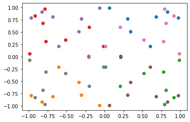
for s in my_group.genpos:
g = symd.str2mat(s)
xp = homo_points @ g
xp = np.fmod(xp, 1.0)
plt.plot(xp[:, 0], xp[:, 1], "o")
plt.show()
Now let’s try applying the special positions, also known as Wyckoff sites.
for sp in my_group.specpos:
    for s in sp.genpos:
        g = symd.str2mat(s)
        xp = homo_points @ g
        xp = np.fmod(xp, 1.0)
        plt.plot(xp[:, 0], xp[:, 1], "o")
plt.show()
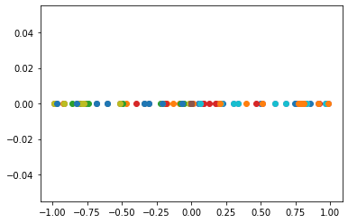
You can see the two sub groups: points on the line and the origin.
Asymmetric unit
As you add more points, you’ll notice that there is overlap:
N = 8000
D = 2
some_points = np.random.rand(N, D)
homo_points = np.concatenate((some_points, np.ones((N, 1))), axis=-1)

for s in my_group.genpos:
    g = symd.str2mat(s)
    xp = homo_points @ g
    xp = np.fmod(xp, 1.0)
    plt.plot(xp[:, 0], xp[:, 1], ".")
plt.show()
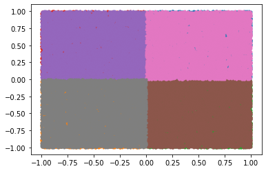
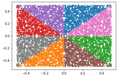
This is because our randomly generated points do not all lie in the asymmetric unit. We can load the asymmetric unit test function and use it to filter our points
in_unit = symd.asymm_constraints(my_group.asymm_unit)
print(in_unit(0.2, -0.3))
print(in_unit(0.2, 0.3))
False
True
# filter out those not in asmmetric unit
some_points = some_points[[in_unit(*p) for p in some_points]]
homo_points = np.concatenate((some_points, np.ones((some_points.shape[0], 1))), axis=-1)

for s in my_group.genpos:
    g = symd.str2mat(s)
    xp = homo_points @ g
    xp = np.fmod(xp, 1.0)
    plt.plot(xp[:, 0], xp[:, 1], ".")
plt.show()
Fractional vs Euclidean Coordinates
All the work above required the points to be between 0 and 1, which are called fractional coordinates. Namely, a value of 0.2, 0.1 means that 20% of lattice vector 1 and 10% of lattice vector 2. How can you can you work with real particles though? You can easily convert via matrix multiplication between fractional coordinates and Euclidean coordintes. In our example above, the Bravais lattice is square so let’s make a square set of lattice vectors to see this:
v1 = [11, 0] # 11 wide
v2 = [0, 3] # 3 tall
B = np.array([v1, v2]).T
print(B)
[[11  0]
 [ 0  3]]
Note that we have the lattice vectors as columns. This makes converting between formats just a matrix multiplication. We can switch back and forth using the inverse of B
Bi = np.linalg.inv(B)

N = 10
some_points = np.random.uniform(-10, 10, size=(N, D))
homo_points = np.concatenate((some_points, np.ones((N, 1))), axis=-1)

# convert to frac coords from Euclidean
frac_coords = some_points @ Bi
# convert back to Eculidean
eucl_coords = frac_coords @ B

plt.plot(some_points[:, 0], some_points[:, 1], "o")
plt.plot(eucl_coords[:, 0], eucl_coords[:, 1], "o", color=None, mec='C2')
plt.show()
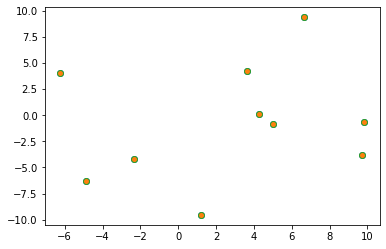
You can see we are able to go to fractional coordinates and back to Euclidean with matrix multiplication. In simulation engines, we also will wrap using np.fmod(frac_coords, 1.0) on the asymetric unit
Bravais Lattice
The Bravais lattice isn’t always square. To get correct lattice vectors, we can use the symd.project_cell function:
lattice_vectors = np.random.uniform(size=(2, 2))
blattice_vectors = symd.project_cell(lattice_vectors, my_group.lattice)
print("This lattice is", my_group.lattice)
print(blattice_vectors)
This lattice is Square
[[1.31528419 0.        ]
 [0.         1.31528419]]
There are a few other convenience functions, like counting the number of particles in a cell if you duplicate for all sites, and getting the cell volume
print("The volume of my cell is", symd.cell_volume(blattice_vectors))
print(
    "If I have 8 particles in asymmetric unit, there will be",
    symd.cell_nparticles(my_group, 8),
    "in the unit cell",
)
print(
    "If I want to have a number density of 0.6 with 8 particles,\nmy cell should be",
    symd.get_cell(0.6, my_group, dim=2, n=8),
)
The volume of my cell is 1.7299725113082867
If I have 8 particles in asymmetric unit, there will be 64 in the unit cell
If I want to have a number density of 0.6 with 8 particles,
my cell should be [5.163977476386403, 0.0, 0.0, 5.163977476386403]