 By
By Input Data & Equivariances
Contents
9. Input Data & Equivariances#
Molecular graphs and structures (xyz coordinates) are the fundamental features in molecules and materials. As discussed, often these are converted into molecular descriptors or some other representation. Why is that? Why can we not work with the data directly? For example, let’s say we have a butane molecule and would like to predict its potential energy from its positions. You could train a linear model \(\hat{E}\) that predicts energy
where \(\textbf{X}\) is \(N\) (14 atoms) \(\times\) \(3\) (xyz coordinates) matrix containing positions, \(\vec{x}\) is a flattened length \(3N\) vector, \(\vec{w}\) is a trainable \(3N\) length vector, and \(b\) is a trainable constant. So far, this is all superficially reasonable – but do not actually use this model, it is wrong in a few ways. Now what if I translate each \(x\), \(y\), \(z\) coordinate by -10:
We know the energy should not change if we translate all the coordinates equally – the molecule is not changing conformations. However, our linear regression will change by \( - 10 \sum \vec{w}\). We have accidentally made our model sensitive to the origin of our coordinate system, which is not physical. This is translational variance – our model changes when we translate the coordinates. I made this word up by the way, no one says that; but it’s just easier to type out than “not translational invariant.” We want our models to be insensitive to this — translationally invariant.
Audience & Objectives
This chapter builds on Graph Neural Networks and a basic knowledge of linear algebra. After completing this chapter, you should be able to
Define invariance vs equivariance
Define translation, rotation, and permutation equivariance
Choose features that have desired invariances
Consider another example from our butane molecule. What if we swapped the order of the atoms in our \(\textbf{X}\) matrix. There is no such thing as a “first” or “second” atom in our molecule, so it should not matter. However, you’ll see that changing the order of \(\textbf{X}\) changes which weights are multiplied and thus the predicted energy will change. This is called a permutation variance. Our model changes if we re-order our inputs, even though from our knowledge of chemistry this should not matter. Similarly, our output energy should not be sensitive to a rotation of the molecular coordinates. Namely they should be permutation invariant and rotationally invariant.
9.1. Equivariances#
Models that work with molecules should be permutation equivariant if they are outputting a per-atom or per-bond quantity. Permutation equivariant means that if you rearrange the order of atoms, the output changes in the same way. For example, if you’re predicting partial charge per atom \(\vec{y} = f(\textbf{X})\) where \( f(\textbf{X})\) is our model function. If you rearrange \(\textbf{X}\), you expect the \(\vec{y}\) to rearrange to match that. Let’s try to state this with an equation. Consider \(\mathcal{P}_{34}\) to be the permutation operator. It swaps indices 3 and 4 in axis 0 of a tensor. Then a permutation equivariant model equation should have:
where \(i,j\) are indices of \(\textbf{X}\) (atom indices). For example, consider \(f(\textbf{X})\) to predict partial charge given a molecule. If the input is water, our input atoms could be arranged HOH and \(f(\textbf{X}) = (0.3, -0.6, 0.3)\). Now if we swap atoms 0 and 1, our input is arranged OHH. If our function is permutation equivariant, then it should output \(f\left(\mathcal{P}_{01}\left[\textbf{X}\right]\right) = \mathcal{P}_{01}\left[\vec{y}\right] = (-0.6, 0.3, 0.3)\).
You can find a more general form of permutation equivariance in [TSK+18]. Now what happens if we output a scalar like energy? Then our permutation operator does nothing:
we call this case a permutation invariance.
Note
An invariance is special type of equivariance. If something is equivariant, you can easily make it invariant (e.g., averaging over your equivariant axes).
9.2. Equivariances of Coordinates#
When we work with molecular coordinates as features we need to be a bit more careful in distinguishing between the “features” that might be element identity and those which specify the location in space. This kind of data is referred to as point clouds in computer science. Let’s break our features into \((\vec{r}, \vec{x})\) where \(\vec{r}\) is the location of the atom/point and \(\vec{x}\) are its features (e.g., element, charge, spin, etc.). Similarly, we may have labels at each point so that we write our labels as \((\vec{r}', \vec{y})\). The label might be direction \(\vec{r}'\) and force magnitude \(y\) or perhaps a field at \(\vec{r}'\) with vectors \(\vec{y}\). You may not have \(\vec{r}'\) like if you’re predicting energy. It may be that \(\vec{r} = \vec{r}'\). With this notation, we can write out translation equivariance as:
You can also write this out if you have a matrix of atom positions (like a molecule):
where \(\textbf{R}\) is the matrix of all position vectors \(\vec{r}_i\). In the case that you do not have output coordinates \(\vec{r}'\), then it becomes:
which we call translation invariance. It’s important to note that these equations do not apply to some specific \(\vec{t}\), but any \(\vec{t}\).
Rotational equivariance can be similarly defined. Consider \(\mathcal{R}\) to be a rotation operator (e.g., a quaternion). Then our rotation equivariance equation is
an example might be again that \((\textbf{R}', \vec{y}_i)\) defines some field and our equivariance says that if we rotate our input points, our output points will obey the same rotation. Again, we can also have rotation invariance if our model does not output \(\textbf{R}'\).
9.3. Constructing Equivariant Models#
There has been some work to unify equivariances into a single “layer” type so that you can just pick what equivariances you want like you would a hyperparameter [TSK+18, WGW+18]. The chapter Equivariant Neural Networks covers these and a recent review may be found in [Est20]. A popular implementation is available here. A recent application in molecules was in predicting dipole moments, a great example of where rotation invariance would fail because dipole moments should rotate the same way when the molecule rotates[MGSNoe20].
If you do not need full equivariances, you can often use a data transformation to make the model invariant regardless of its architecture. Some of the common transforms are summarized in the table below and you can find a much more detailed discussion of data transformations in Musil et al. [MGB+21]. The list below omits data augmentation where you try to teach your model these invariances through training — which is a common and effective strategy in image deep learning. Alternatively, if your invariants are finite (e.g., only 90 degree rotations or you have small permutation invariant sets) you can just apply each possible transformation (rotation/permutation) and average the results to make a quick and easy invariant network[ZKR+17]. That is sometimes called test augmentation.
Data Transformation |
Equivariance |
|---|---|
Matrix Determinant |
Permutation Invariance |
Eigendecomposition |
Permutation Invariance |
Reduction (sum, mean) |
Permutation Invariance |
Pairwise Vector/Distance |
Translation/Rotation Invariance |
Angles |
Translation/Rotation Invariance |
Atom-centered Symmetry Functions |
Rotation/Translation Invariance |
Trajectory Alignment |
Rotation/Translation Invariance |
Molecular Descriptors |
All invariant |
9.3.1. Matrix Determinant#
A matrix determinant is not quite permutation invariant. If you swap two rows in a matrix, it makes the determinant change signs. However, you can easily just square the determinant to remove the sign change. How would you use a determinant in a model? It’s just a building block. You could build a matrix of all neighbor features in a molecular graph and then do a determinant to arrive at a permutation invariant output. The determinant has two major disadvantages: (i) it outputs a single number (not that expressive) and (ii) it’s really expensive \(O(n^3)\). Thus you won’t see a determinant too frequently in deep learning.
9.3.2. Eigendecomposition#
The eigendecomposition is when you factorize a matrix into its eigenvalues and eigenvectors. The (sorted) eigenvalues of a matrix are permutation invariant. Compared with the determinant, you get more eigenvalues from a matrix than determinants so there is less loss of information. Computing eigenvalues is still expensive at \(O(n^3)\) and they are not differentiable. Nevertheless, you will see this strategy in kernel learning where you do not need to propagate derivatives through the kernel. One important application of this is in some of the early work on quantum machine learning [RTMullerVL12].
9.3.3. Reductions#
An obvious way to remove permutation variance is to just sum over the points or atoms. More generally, you can use any kind of reduction like a mean or product. Like a determinant, this results in a single number or at least removal of an axis. Reductions are fast and differentiable.
9.3.4. Pairwise Distance#
Using pairwise distances or vectors is the standard solution to translation invariance. Rarely are we actually that concerned with translational equivariance. If using pairwise vectors between atoms instead of the xyz coordinates, this naturally removes the choice of origin and thus makes the model translation invariant. If we go further and use pairwise distance instead of vectors, this also removes the effect of rotations giving a rotation invariance. This is fast, differentiable, and the usual approach to add translation and rotation invariance.
9.3.5. Angles#
Angles are rotation, translation, and scale invariant. You can define angles any way, but often they are done between consecutive bonds (3 atoms total). Combining angles and pairwise distances (along bonds only) are called internal coordinates.
9.3.6. Convolutional Layers#
Convolutional layers are well-known to be translationally equivariant. Remember that they work in 3D as well, so they can be an input layer if translational equivariance is desired. However, convolutions work on pixels or voxels in 3D, so you must first bin your coordinates into a voxel grid. See Chew et al. for an example [CJZ+20].
9.3.7. Atom-centered Symmetry Functions#
These are a large class of functions described by Behler[Beh11] that transform from the input coordinate/features \((\mathbf{R}, \mathbf{X})\) to a new set of features \(\mathbf{X}'\) that obey rotational and translational symmetry. This makes them translational and rotationally invariant. Behler didn’t propose a single function to get these features, but instead explored the choices and theory. Bartók et al. [BartokKCsanyi13] provided a specific recipe which is called a SOAP descriptor. These are drop-in replacements for \((\mathbf{R}, \mathbf{X})\) that are translation and rotation invariant but do not lose much information. They are differentiable, although complex to implement.
9.3.8. Trajectory Alignment#
One special case is when your points are part of a time-dependent trajectory. This usually implies that the order of the points does not change. Thus, we do not need to worry about permutation invariance. This is the case when analyzing results from a molecular dynamics trajectory, like a dynamic simulation of a protein. One way to make our data translation and rotation invariant in this case is to align it to some reference coordinates. For example, you could always make the center of mass of the trajectory be at the origin. This will make the points translation invariant, because you always center a new set of points. A natural question is if it must be the center of mass? No, because your points are permutation invariant, you could just pick point 0 as the origin. Then if the points are translated, this will be undone when you move the points such that point 0 is the origin. To be more precise, we always apply a centering function \(c\left(\mathbf{R}\right)\) that redefines the origin before processing a set of points. We can also define a rotation function \(r\left(\mathbf{R}\right)\) that will be applied where we align to some definite set of three Euler angles (two vectors). See the example below for this.
9.3.9. Molecular Descriptors#
Molecular descriptors are the classic way to convert molecules into translation/rotation/permutation invariant features. There exists 3D descriptors as well that can treat structure. They are also called fingerprints. Fingerprints is a broad term for converting a molecular structure to a binary sequence. Commonly, each bit indicates the presence or absence of a specific substructure. We won’t focus on these in this course because they are untrainable and choosing the correct combination of descriptors is an unsolved problem which has no clear process.
9.4. Examples#
Let’s demonstrate with some code how to go about creating functions that obey these equivariances. We won’t be training these models because training has no effect on equivariances, but you should train your models if you’re doing learning 😉
I’ll define my butane molecule as a set of coordinates \(\mathbf{R}_i\) and features \(\mathbf{X}_i\). My features are just one-hot vectors indicating if a particular point is a carbon atom \([1,0]\) or a hydrogen atom \([0,1]\). In our example, we will just be interested in predicting energy. We will not train our models, so the energy will not be accurate.
9.5. Running This Notebook#
Click the above to launch this page as an interactive Google Colab. See details below on installing packages.
Tip
To install packages, execute this code in a new cell.
!pip install dmol-book
If you find install problems, you can get the latest working versions of packages used in this book here
import numpy as np

R_i = np.array(
    [
        -0.5630,
        0.5160,
        0.0071,
        0.5630,
        -0.5159,
        0.0071,
        -1.9293,
        -0.1506,
        -0.0071,
        1.9294,
        0.1505,
        -0.0071,
        -0.4724,
        1.1666,
        -0.8706,
        -0.4825,
        1.1551,
        0.8940,
        0.4825,
        -1.1551,
        0.8940,
        0.4723,
        -1.1665,
        -0.8706,
        -2.0542,
        -0.7710,
        -0.9003,
        -2.0651,
        -0.7856,
        0.8742,
        -2.7203,
        0.6060,
        -0.0058,
        2.0542,
        0.7709,
        -0.9003,
        2.7202,
        -0.6062,
        -0.0059,
        2.0652,
        0.7854,
        0.8743,
    ]
).reshape(-1, 3)
N = R_i.shape[0]
X_i = np.zeros((N, 2))
X_i[:4, 0] = 1
X_i[4:, 1] = 1
9.5.1. No equivariances#
A one-hidden layer dense neural network is an example of a model with no equivariances. To fit our data into this dense layer, we’ll just stack the positions and features into a large input tensor and output energy. We’ll use a tanh as activation, 16 hidden layer dimension, and our output layer has no activation because we’re doing regression to energy. Our weights will always be randomly initialized.
# our 1-hidden layer model
def hidden_model(r, x, w1, w2, b1, b2):
    # stack into one large input
    i = np.concatenate((r, x), axis=1).flatten()
    v = np.tanh(i @ w1 + b1)
    v = v @ w2 + b2
    return v


# initialize our weights
w1 = np.random.normal(size=(N * 5, 16))  # 5 -> 3 xyz + 2 features
b1 = np.random.normal(size=(16,))
w2 = np.random.normal(size=(16,))
b2 = np.random.normal()
Let’s see what the predicted energy is with our coordinates.
hidden_model(R_i, X_i, w1, w2, b1, b2)
-0.15661844175945916
This is not trained, so we aren’t that concerned about the value. Now let’s see if our model is sensitive to translation.
hidden_model(R_i + np.array([1, 2, 3]), X_i, w1, w2, b1, b2)
-2.28169204607694
As expected, it is sensitive to translation. I added the vector \((1, 2, 3)\) to all input points and the energy changed. This model is not translation invariant. The choice of \((1,2,3)\) is arbitrary, the model should not change output regardless of the choice of the translation vector if the model is translation invariant. Rotations can be done using the scipy.transformation library which takes care of some of the messiness of working with quaternions, which are the operators that perform rotations.
import scipy.spatial.transform as trans

# rotate around x coord by 45 degrees
rot = trans.Rotation.from_euler("x", 45, degrees=True)

print("No rotation", hidden_model(R_i, X_i, w1, w2, b1, b2))
print("Rotated", hidden_model(rot.apply(R_i), X_i, w1, w2, b1, b2))
No rotation -0.15661844175945916
Rotated -5.119274714081461
Our model is affected by the rotation, meaning it is not rotation invariant. Permutation invariance comes from swapping indices.
# swap 0, 1 rows
perm_R_i = np.copy(R_i)
perm_R_i[0], perm_R_i[1] = R_i[1], R_i[0]
# we do not need to swap X_i 0,1 because they are identical

print("original", hidden_model(R_i, X_i, w1, w2, b1, b2))
print("permuted", hidden_model(perm_R_i, X_i, w1, w2, b1, b2))
original -0.15661844175945916
permuted 0.03127964078571854
Our model is not permutation invariant!
9.5.2. Permutation Invariant#
We will use a reduction to achieve permutation invariance. All that is needed is to ensure that weights are not a function of our atom number axis and then do a reduction (sum) prior to the output layer. Here is the implementation.
# our 1-hidden layer model with perm inv
def hidden_model_pi(r, x, w1, w2, b1, b2):
    # stack into one large input
    i = np.concatenate((r, x), axis=1)
    v = np.tanh(i @ w1 + b1)
    # reduction
    v = np.sum(v, axis=0)
    v = v @ w2 + b2
    return v


# initialize our weights
w1 = np.random.normal(size=(5, 16))  # note it no lonegr has N!
b1 = np.random.normal(size=(16,))
w2 = np.random.normal(size=(16,))
b2 = np.random.normal()
We made three changes: we kept the atom axis (no more flatten), we removed the atom axis after the hidden layer (sum), and we made our weights not depend on the atom axis. Now let’s observe if this is indeed permutation invariant.
print("original", hidden_model_pi(R_i, X_i, w1, w2, b1, b2))
print("permuted", hidden_model_pi(perm_R_i, X_i, w1, w2, b1, b2))
original -2.8563726750717713
permuted -2.8563726750717713
It is!
9.5.3. Translation Invariant#
The next change we will make is to convert our \(N\times3\) shaped coordinates into \(N\times N\times 3\) pairwise vectors. This gives us translation invariance. This causes an issue because our distance features went from being \(3\) per atom to \(N \times 3\) per atom. Thus we’ve introduced a dependence on atom number in our distance features and that means it’s easy to accidentally break our permutation invariance. We can just sum over this new axis though. Let’s see an implementation:
# our 1-hidden layer model with perm inv, trans inv
def hidden_model_pti(r, x, w1, w2, b1, b2):
    # compute pairwise distances using broadcasting
    d = r - r[:, np.newaxis]
    # stack into one large input of N x N x 5
    # concatenate doesn't broadcast, so I manually broadcast the Nx2 x matrix
    # into N x N x 2
    i = np.concatenate((d, np.broadcast_to(x, (d.shape[:-1] + x.shape[-1:]))), axis=-1)
    v = np.tanh(i @ w1 + b1)
    # reduction over both axes
    v = np.sum(v, axis=(0, 1))
    v = v @ w2 + b2
    return v
print("original", hidden_model_pti(R_i, X_i, w1, w2, b1, b2))
print("permuted", hidden_model_pti(perm_R_i, X_i, w1, w2, b1, b2))
print("translated", hidden_model_pti(R_i + np.array([-2, 3, 4]), X_i, w1, w2, b1, b2))
print("rotated", hidden_model_pti(rot.apply(R_i), X_i, w1, w2, b1, b2))
original -50.87198674851824
permuted -50.87198674851826
translated -50.87198674851826
rotated -54.67158374882283
It is now translation and permutation invariant. But not yet rotation invariant.
9.5.4. Rotation Invariant#
It is a simple change to make it rotationally invariant. We just convert the pairwise vectors into pairwise distances. We’ll use squared distances for simplicity.
# our 1-hidden layer model with perm, trans, rot inv.
def hidden_model_ptri(r, x, w1, w2, b1, b2):
    # compute pairwise distances using broadcasting
    d = r - r[:, np.newaxis]
    # x^2 + y^2 + z^2 of pairwise vectors
    # keepdims so we get an N x N x 1 output
    d2 = np.sum(d**2, axis=-1, keepdims=True)
    # stack into one large input of N x N x 3
    # concatenate doesn't broadcast, so I manually broadcast the Nx2 x matrix
    # into N x N x 2
    i = np.concatenate(
        (d2, np.broadcast_to(x, (d2.shape[:-1] + x.shape[-1:]))), axis=-1
    )
    v = np.tanh(i @ w1 + b1)
    # reduction over both axes
    v = np.sum(v, axis=(0, 1))
    v = v @ w2 + b2
    return v


# initialize our weights
w1 = np.random.normal(size=(3, 16))  # now just 1 dist feature
b1 = np.random.normal(size=(16,))
w2 = np.random.normal(size=(16,))
b2 = np.random.normal()

# test it

print("original", hidden_model_ptri(R_i, X_i, w1, w2, b1, b2))
print("permuted", hidden_model_ptri(perm_R_i, X_i, w1, w2, b1, b2))
print("translated", hidden_model_ptri(R_i + np.array([-2, 3, 4]), X_i, w1, w2, b1, b2))
print("rotated", hidden_model_ptri(rot.apply(R_i), X_i, w1, w2, b1, b2))
original -207.3246711060532
permuted -207.32467110605322
translated -207.3246711060532
rotated -207.32467110605322
We have achieved our invariances! Remember that you could use different choices to achieve these invariances. Also, you may not want an invariance sometimes. You may want equivariances or are not concerned at all. For example, if you’re always working with one molecule you may never need to switch around atom orders.
Finally as a sanity check, let’s make sure that if we change the coordinates our predicted energy changes.
R_i[0] = 2.0
print("changed", hidden_model_ptri(R_i, X_i, w1, w2, b1, b2))
changed -222.58046782961173
Our model is still sensitive to the input features
9.6. Trajectory Alignment Example#
As described above, if you’re working with a trajectory there is no requirement to have permutation equivariance. To achieve translation and rotation invariance, we can align to some fixed points that will be present in all structures (like center of mass). As we’ll see below, trajectory alignment is fraught with issues like rotation ambiguities, unphysical rotations, and creating fictitious covariances between far away points due to alignment. Internal coordinates (pairwise dist, angles) are almost always better. However, trajectory alignment has good scaling properties.
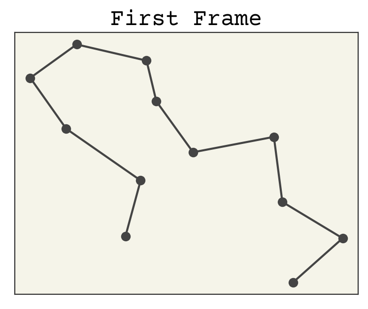
The movie below shows an example trajectory that we’ll examine. I’ve made it 2D to make it simple to visualize, but the same principles apply to 3D.
Let’s start by loading the trajectory and defining/testing our centering function. The trajectory is a tensor that is shape time, point number, xy -> (2048, 12, 2). I’ll examine two centering functions: align to center of mass and align to point 0 to see what the two look like.
# new imports
import matplotlib.pyplot as plt
import urllib
import dmol
urllib.request.urlretrieve(
    "https://github.com/whitead/dmol-book/raw/main/data/paths.npz", "paths.npz"
)
paths = np.load("paths.npz")["arr"]
# plot the first point
plt.title("First Frame")
plt.plot(paths[0, :, 0], paths[0, :, 1], "o-")
plt.xticks([])
plt.yticks([])
plt.show()
def center_com(paths):
    """Align paths to COM at each frame"""
    coms = np.mean(paths, axis=-2, keepdims=True)
    return paths - coms


def center_point(paths):
    """Align paths to particle 0"""
    return paths - paths[:, :1]


ccpaths = center_com(paths)
cppaths = center_point(paths)
To compare, we’ll draw a sample of frames on top of one another to see the now translationally invariant coordinates.
fig, axs = plt.subplots(ncols=3, squeeze=True, figsize=(16, 4))

axs[0].set_title("No Center")
axs[1].set_title("COM Center")
axs[2].set_title("Point 0 Center")
cmap = plt.get_cmap("cool")
for i in range(0, 2048, 16):
    axs[0].plot(paths[i, :, 0], paths[i, :, 1], ".-", alpha=0.2, color=cmap(i / 2048))
    axs[1].plot(
        ccpaths[i, :, 0], ccpaths[i, :, 1], ".-", alpha=0.2, color=cmap(i / 2048)
    )
    axs[2].plot(
        cppaths[i, :, 0], cppaths[i, :, 1], ".-", alpha=0.2, color=cmap(i / 2048)
    )
for i in range(3):
    axs[i].set_xticks([])
    axs[i].set_yticks([])
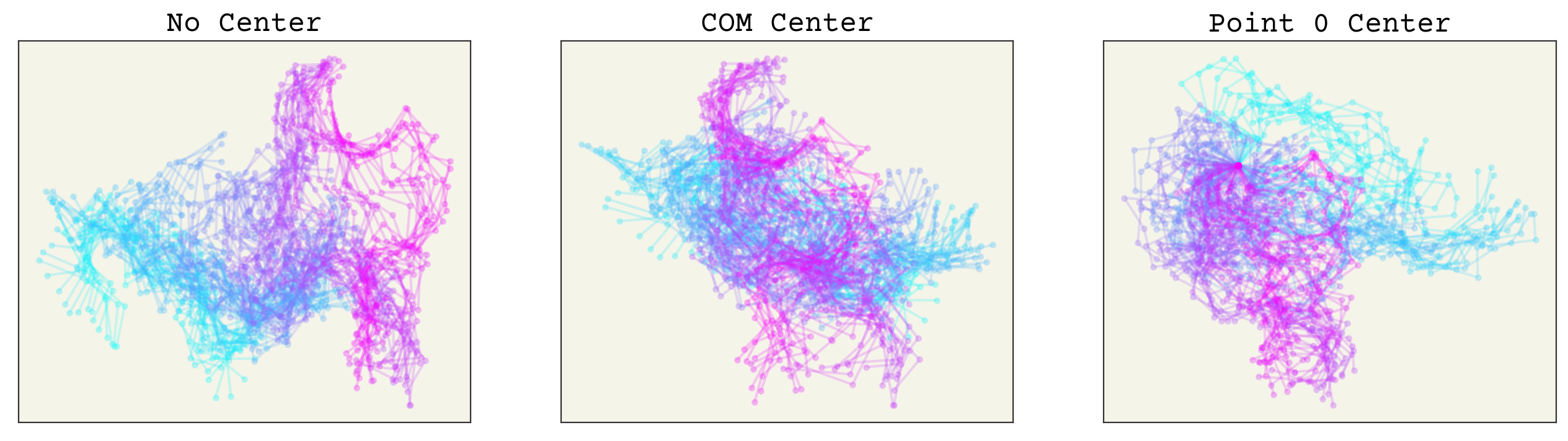
The color indicates time. You can see that having no alignment makes the spatial coordinates depend on time implicitly because the points drift over time. Both aligning to COM or point 0 removes this effect. The COM implicitly removes 2 degrees of freedom. Point 0 alignment makes point 0 have no variance (also remove degrees of freedom), which could affect how you design or interpret your model.
Now we will align by rotation. We need to define a unique rotation. A simple way is to choose 1 (or 2 in 3D) vectors that define our coordinate system directions. For example, we could choose that the vector from point 0 to point 1 defines the positive direction of the x-axis. A more sophisticated way is to find the principal axes of our points and align along these. For 2D, we only need to align to one of them. Again, this implicitly removes a degree of freedom. We will examine both. Computing principle axes requires an eigenvalue decomposition, so it’s a bit more numerically intense [FR00].
Warning
For all rotation alignment methods, you must have already centered the points.
def make_2drot(angle):
    mats = np.array([[np.cos(angle), -np.sin(angle)], [np.sin(angle), np.cos(angle)]])
    # swap so batch axis is first
    return np.swapaxes(mats, 0, -1)


def align_point(paths):
    """Align to 0-1 vector assuming 2D data"""
    vecs = paths[:, 0, :] - paths[:, 1, :]
    # find angle to rotate so these are pointed towards pos x
    cur_angle = np.arctan2(vecs[:, 1], vecs[:, 0])
    rot_angle = -cur_angle
    rot_mat = make_2drot(rot_angle)
    # to mat mult at each frame
    return paths @ rot_mat


def find_principle_axis(points, naxis=2):
    """Compute single principle axis for points"""
    inertia = points.T @ points
    evals, evecs = np.linalg.eig(inertia)
    order = np.argsort(evals)[::-1]
    # return largest vectors
    return evecs[:, order[:naxis]].T


def align_principle(paths, axis_finder=find_principle_axis):
    # someone should tell me how to vectorize this in numpy
    vecs = [axis_finder(p) for p in paths]
    vecs = np.array(vecs)
    # find angle to rotate so these are pointed towards pos x
    cur_angle = np.arctan2(vecs[:, 0, 1], vecs[:, 0, 0])
    cross = np.cross(vecs[:, 0], vecs[:, 1])
    rot_angle = -cur_angle - (cross < 0) * np.pi
    rot_mat = make_2drot(rot_angle)
    # rotate at each frame
    rpaths = paths @ rot_mat
    return rpaths


appaths = align_point(cppaths)
apapaths = align_principle(ccpaths)
fig, axs = plt.subplots(ncols=3, squeeze=True, figsize=(16, 4))

axs[0].set_title("No Align")
axs[1].set_title("COM Align")
axs[2].set_title("Point 0 Align")
for i in range(0, 2048, 16):
    axs[0].plot(paths[i, :, 0], paths[i, :, 1], ".-", alpha=0.2, color=cmap(i / 2048))
    axs[1].plot(
        apapaths[i, :, 0], apapaths[i, :, 1], ".-", alpha=0.2, color=cmap(i / 2048)
    )
    axs[2].plot(
        appaths[i, :, 0], appaths[i, :, 1], ".-", alpha=0.2, color=cmap(i / 2048)
    )
for i in range(3):
    axs[i].set_xticks([])
    axs[i].set_yticks([])
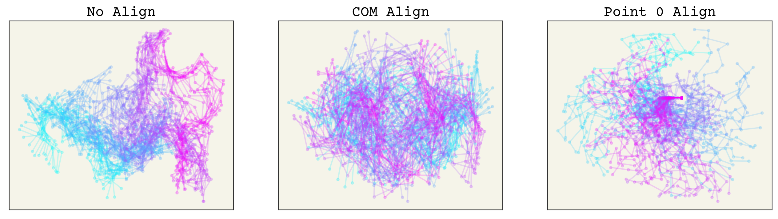
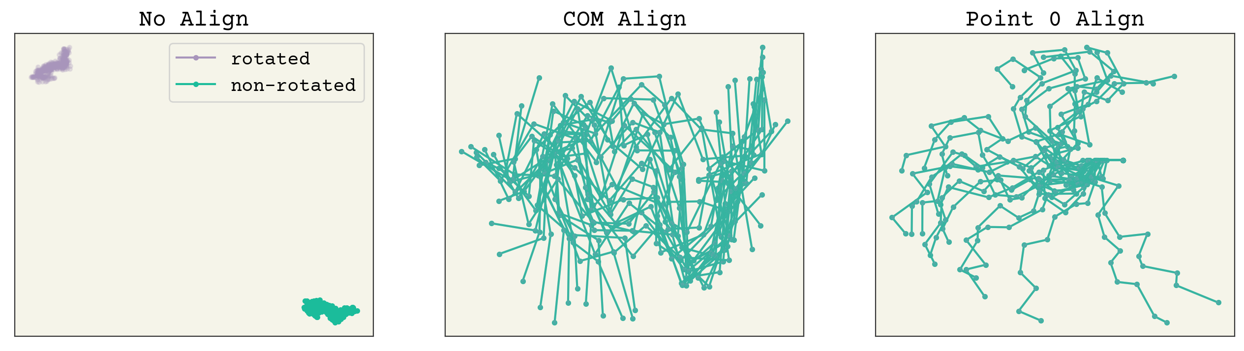
You can see how points far away on the chain from 0 have much more variance in the point 0 align, whereas the COM alignment looks better spread. Remember, to apply these methods you must do them to both your training data and any prediction points. Thus, they should be viewed as part of your neural network. We can now check that rotating has no effect on these. The plots below have the trajectory rotated by 1 radian and you can see that both alignment methods have no change (the lines are overlapping).
rot_paths = paths @ make_2drot(1)
rot_appaths = align_point(center_point(rot_paths))
rot_apapaths = align_principle(center_com(rot_paths))
fig, axs = plt.subplots(ncols=3, squeeze=True, figsize=(16, 4))

axs[0].set_title("No Align")
axs[1].set_title("COM Align")
axs[2].set_title("Point 0 Align")
for i in range(0, 500, 20):
    axs[0].plot(paths[i, :, 0], paths[i, :, 1], ".-", alpha=1, color="C1")
    axs[1].plot(apapaths[i, :, 0], apapaths[i, :, 1], ".-", alpha=1, color="C1")
    axs[2].plot(appaths[i, :, 0], appaths[i, :, 1], ".-", alpha=1, color="C1")
    axs[0].plot(rot_paths[i, :, 0], rot_paths[i, :, 1], ".-", alpha=0.2, color="C2")
    axs[1].plot(
        rot_apapaths[i, :, 0], rot_apapaths[i, :, 1], ".-", alpha=0.2, color="C2"
    )
    axs[2].plot(rot_appaths[i, :, 0], rot_appaths[i, :, 1], ".-", alpha=0.2, color="C2")
# plot again to get handles
axs[0].plot(np.nan, np.nan, ".-", alpha=1, color="C2", label="rotated")
axs[0].plot(np.nan, np.nan, ".-", alpha=1, color="C1", label="non-rotated")
axs[0].legend()
for i in range(3):
    axs[i].set_xticks([])
    axs[i].set_yticks([])
Now which method is better? Aligning based on arbitrary points is indeed easier, but it creates an unusual new variance in your features. For example, let’s see what happens if we make a small perturbation to one conformation. The code is hidden for simplicity. We try changing point 1, then point 0, then point 11 to see the effects of perturbations along the chain.
NP = 16


def perturb_paths(perturb_point):
    perturbation = np.zeros_like(paths[:NP])
    perturbation[:, perturb_point, 0] = np.linspace(0, 0.2, NP)
    test_paths = paths[0:1] - perturbation

    # compute aligned trajs
    appaths = align_point(center_point(test_paths))
    apapaths = align_principle(center_com(test_paths))

    fig, axs = plt.subplots(ncols=3, squeeze=True, figsize=(16, 4))
    axs[0].set_title(f"Perturb {perturb_point} - No Align")
    axs[1].set_title(f"Perturb {perturb_point} - COM Align")
    axs[2].set_title(f"Perturb {perturb_point} - Point 0 Align")
    for i in range(NP):
        axs[0].plot(
            test_paths[i, :, 0],
            test_paths[i, :, 1],
            ".-",
            alpha=0.2,
            color=cmap(i / NP),
        )
        axs[1].plot(
            apapaths[i, :, 0], apapaths[i, :, 1], ".-", alpha=0.2, color=cmap(i / NP)
        )
        axs[2].plot(
            appaths[i, :, 0], appaths[i, :, 1], ".-", alpha=0.2, color=cmap(i / NP)
        )
    for i in range(3):
        axs[i].set_xticks([])
        axs[i].set_yticks([])


perturb_paths(0)
perturb_paths(1)
perturb_paths(11)
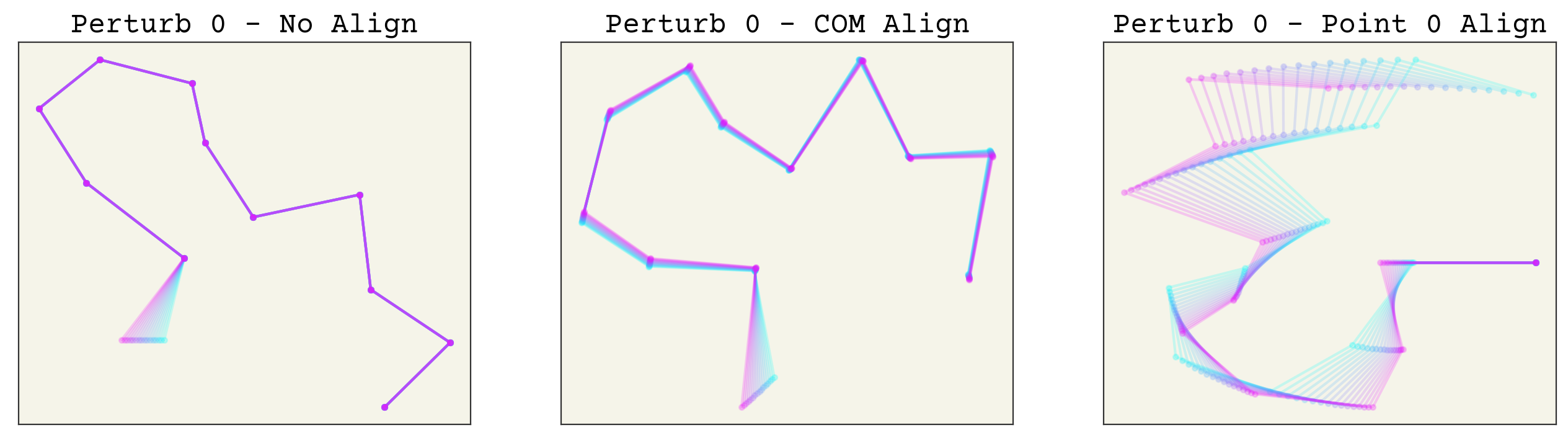
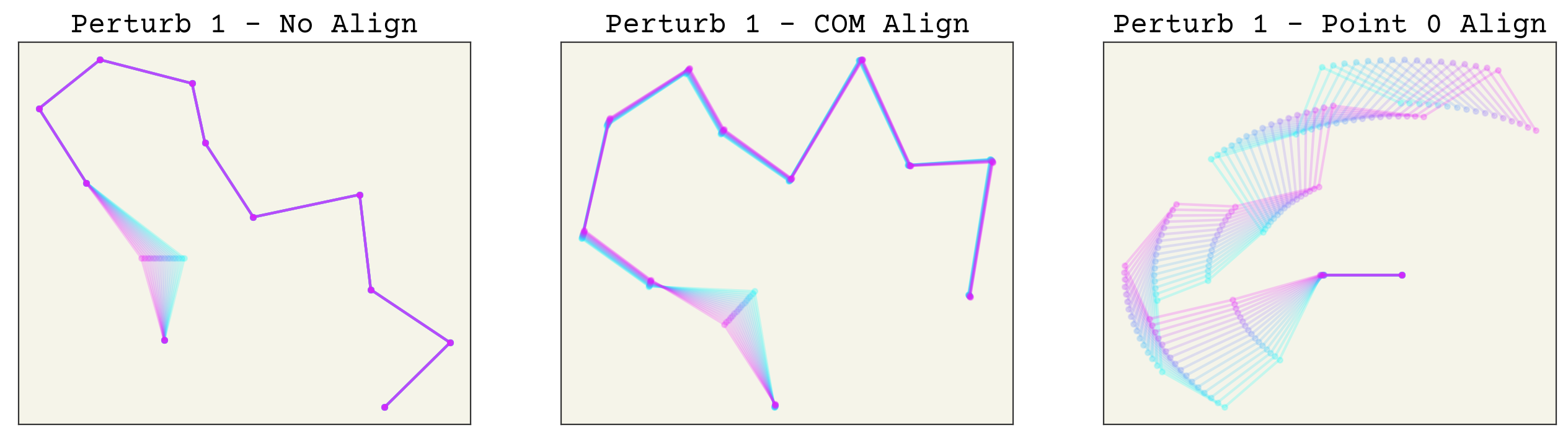
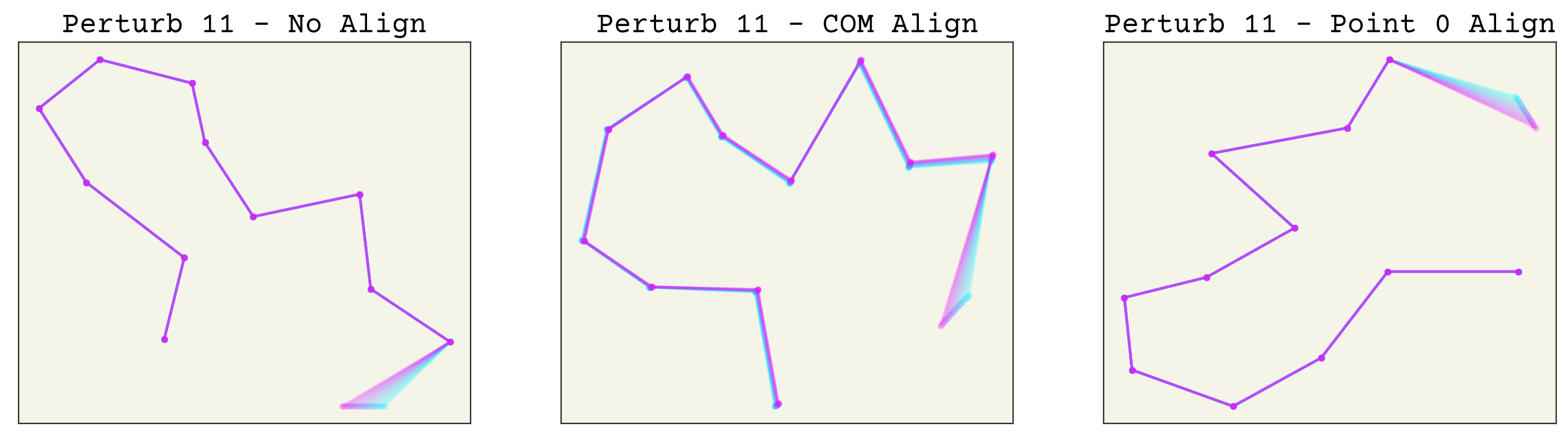
As you can see, perturbing one point alters all others after alignment. This makes these transformed features sensitive to noise, especially aligning to point 0 or 1. More importantly, this effect is uneven in the alignment to point 0. This can in-turn make training quite difficult. Of course, neural networks are universal approximators so in theory this should not matter. However, I expect that using the COM alignment approach will give better training because the network will not need to account for this unusual variance structure.
The final analysis shows a video of the two frames. One thing you’ll note are the jumps, when the principle axes swap direction. You can see that the ambiguity caused by these can create artifacts.
9.6.1. Using Unsupervised Methods for Alignment#
There are additional methods for aligning trajectories. You could define one frame as the “reference” and find the translation and rotations that best align with that reference. This could give some interpretability to your rotation and translation alignment. A tempting option is to use dimensionality reduction (like PCA), but these are not rotation invariant. This is confusing at first, because remember PCA should remove translation and rotation. It removes it though from the training data and not an arbitrary frame because it examines motion along a trajectory. You can easily see this getting principle components and then trying to align a new frame to them and a rotated version of the new frame. You’ll get different results. Another important consideration is if the unsupervised method can handle new data. Manifold embeddings do not provide a linear transform that can handle new data for inference. Manifold embeddings are also not necessarily rotation invariant or equivariant.
9.7. Distance Features#
One more topic on parsing data is treating distances. As we saw above, pairwise distance is a wise transformation because it is translation and rotation invariant. However, we may want to sometimes transform this further. One obvious choice is to use \(1 / r\) as the input to our neural network. This is because most properties of atoms (and thus molecules) are affected by their closest nearby atoms. An oxygen nearby a carbon is much more important than an oxygen that is 100 nanometers away. Choosing \(1 / r\) as an input makes it easier for a neural network to train because it encodes this physical insight about local interactions being the most important. Of course, a neural network could learn to turn \(r\) into \(1/r\) because they are universal approximators. Yet this approach means we do not need to waste training data and weights on learning to change \(r\) into \(1 / r\). This approach will not work on non-local or mildly-non-local effects like electrostatics or multi-scale phenomena.
Another detail on distances is that we often want to “featurize” them; we’d like to go from one a single number like \(r = 3.2\) to a vector of reals. Why? Well that’s just how neural networks learn. Hidden-layers need to have more than 1 dimension to be expressive enough to model any function. This seems like an obvious point though: if you used \(r\) in a neural network it would obviously get larger as it goes through hidden layers. However, there are a few “standard” ways that people like to do this process. There are valid reasons, like making it smoothly differentiable, that you might choose one of these special “featurizing” functions.
9.7.1. Repeating#
The first approach is to just repeat \(r\) up to the desired hidden dimension. This is representable as a dense neural network with no activation.
9.7.2. Binning#
As explored in Gilmer et al. [GSR+17] and others, you can bin your distances to be a one-hot vector. Essentially, you histogram \(r\) into fixed bins so that you only have one bin being “hot”. Each bin will represent a segment of positions (e.g., 4.5-5.0). This has discontinuous derivatives with respect to distance and is rarely used.
9.7.3. Radial Basis Functions#
Radial basis functions are a commonly used procedure for converting a scalar into a fixed number of features and were first used in interpolation[Pow77]. Radial basis functions use the following equation:
where \(d_i\) is an equally spaced vector of distances (e.g., \([1.5, 3.0, 4.5, 6.0]\)) and \(w\) is a trainable (or hyper) parameter. This computes a Gaussian kernel between \(r\) and all distances \(d_i\). What is nice about this expression is the smooth well-behaved derivatives with respect to \(r\) and lack of trainable parameters. You can (almost) represent this with a dense layer and a softmax activation.
9.7.4. Sub NN#
Another strategy used in Gilmer et al. [GSR+17] is to just put your distances through a series of dense layers to get features. For example, if you’re going to use the distance in a graph neural network you could run it through three dense layers first to get a larger feature dimension. Remember that repeating and radial basis functions are equivalent to dense layers (assuming correct activation choice), so this strategy can be a simple solution to the above choice.
9.8. Chapter Summary#
Machine learning models that work with molecules must be permutation invariant, such that if the atoms are rearranged, the output will not change.
Translational invariance of molecular coordinates is when the coordinates are shifted and the resulting output does not change.
Rotational invariance is similar, except the molecular coordinates are rotated.
Data augmentation is when you try to teach your model the various types of equivariances by rotating and translating your training data to create additional examples.
There are various techniques, such as eigendecomposition or pairwise distance to make molecular coordinates invariant.
A one-hidden layer dense neural network is an example of a model with no equivariances.
You can try alignment for trajectories, where each training example has the same ordering and number of atoms.
9.9. Cited References#
- RTMullerVL12
Matthias Rupp, Alexandre Tkatchenko, Klaus-Robert Müller, and O Anatole Von Lilienfeld. Fast and accurate modeling of molecular atomization energies with machine learning. Physical review letters, 108(5):058301, 2012.
- GSR+17(1,2)
Justin Gilmer, Samuel S Schoenholz, Patrick F Riley, Oriol Vinyals, and George E Dahl. Neural message passing for quantum chemistry. arXiv preprint arXiv:1704.01212, 2017.
- ZKR+17
Manzil Zaheer, Satwik Kottur, Siamak Ravanbakhsh, Barnabas Poczos, Russ R Salakhutdinov, and Alexander J Smola. Deep sets. In Advances in neural information processing systems, 3391–3401. 2017.
- TSK+18(1,2)
Nathaniel Thomas, Tess Smidt, Steven Kearnes, Lusann Yang, Li Li, Kai Kohlhoff, and Patrick Riley. Tensor field networks: rotation-and translation-equivariant neural networks for 3d point clouds. arXiv preprint arXiv:1802.08219, 2018.
- WGW+18
Maurice Weiler, Mario Geiger, Max Welling, Wouter Boomsma, and Taco S Cohen. 3d steerable cnns: learning rotationally equivariant features in volumetric data. In Advances in Neural Information Processing Systems, 10381–10392. 2018.
- Est20
Carlos Esteves. Theoretical aspects of group equivariant neural networks. arXiv preprint arXiv:2004.05154, 2020.
- MGSNoe20
Benjamin Kurt Miller, Mario Geiger, Tess E Smidt, and Frank Noé. Relevance of rotationally equivariant convolutions for predicting molecular properties. arXiv preprint arXiv:2008.08461, 2020.
- MGB+21
Felix Musil, Andrea Grisafi, Albert P. Bartók, Christoph Ortner, Gábor Csányi, and Michele Ceriotti. Physics-inspired structural representations for molecules and materials. arXiv preprint arXiv:2101.04673, 2021.
- CJZ+20
Alex K Chew, Shengli Jiang, Weiqi Zhang, Victor M Zavala, and Reid C Van Lehn. Fast predictions of liquid-phase acid-catalyzed reaction rates using molecular dynamics simulations and convolutional neural networks. Chemical Science, 11(46):12464–12476, 2020.
- Beh11
Jörg Behler. Atom-centered symmetry functions for constructing high-dimensional neural network potentials. The Journal of chemical physics, 134(7):074106, 2011.
- BartokKCsanyi13
Albert P. Bartók, Risi Kondor, and Gábor Csányi. On representing chemical environments. Phys. Rev. B, 87:184115, May 2013. URL: https://link.aps.org/doi/10.1103/PhysRevB.87.184115, doi:10.1103/PhysRevB.87.184115.
- RSPoczos17
Siamak Ravanbakhsh, Jeff Schneider, and Barnabás Póczos. Equivariance through parameter-sharing. In International Conference on Machine Learning, 2892–2901. 2017.
- FR00
Jefferson Foote and Anandi Raman. A relation between the principal axes of inertia and ligand binding. Proceedings of the National Academy of Sciences, 97(3):978–983, 2000.
- Pow77
Michael James David Powell. Restart procedures for the conjugate gradient method. Mathematical programming, 12(1):241–254, 1977.