1. Introduction to Deep Learning¶

Deep learning is a category of machine learning. Machine learning is a category of artificial intelligence. These notes are mostly about deep learning, thus the name of the book. Deep learning is the use of neural networks to classify and regress data (this is too narrow, but a good starting definition). I am a chemical engineering professor though; please read more beyond this introduction because my perspective is biased towards chemistry and materials. I found the introduction the from Ian Goodfellow’s book to be a good intro. If you’re more visually oriented, Grant Sanderson has made a short video series specifically about neural networks that give an applied introduction to the topic. DeepMind has a high-level video showing what can be accomplished with deep learning & AI. When people write “deep learning is a powerful tool” in their research papers, they typically cite this Nature paper by Yann LeCun, Yoshua Bengio, and Geoffery Hinton. Zhang, Lipton, Li, and Smola have written a practical and example-driven online book that gives each example in Tensorflow, PyTorch, and MXNet. You can find many chemistry specific examples and information about deep learning in chemistry via the excellent DeepChem project.

The main advice I would give to beginners in deep learning are to focus less on the neurological inspired language (i.e., connections between neurons), and instead view deep learning as a series of linear algebra operations where many of the matrices are filled with adjustable parameters. There are of course a few non-linear functions (activations) here and there, but deep learning is essentially linear algebra operations specified via a “computation network” (aka computation graph) that vaguely looks like neurons connected in a brain.

1.1. Neural Networks¶

The deep in deep learning means we have many layers in our neural networks. What is a neural network? Without loss of generality, we can view neural networks as 2 components: (1) a non-linear function \(g(\cdot)\) which operates on our input features \(\mathbf{X}\) and outputs a new set of features \(\mathbf{H} = g(\mathbf{X})\) and (2) a linear model like we saw in our Introduction to Machine Learning. Our model equation for deep learning regression is:

(1.20)¶\[\begin{equation} \hat{y} = \vec{w}g(\vec{x}) + b \end{equation}\]

One of the main discussion points in our ML chapters was how arcane and difficult it is to choose features. Here, we have replaced our features with a set of trainable features \(g(\vec{x})\) and then use the same linear model as before. So how do we design \(g(\vec{x})\)? That is the deep learning part. \(g(\vec{x})\) is a differentiable function we design composed of layers, which are themselves differentiable functions each with trainable weights (free variables). Deep learning is a mature field and there is a set of standard layers, each with a different purpose. For example, convolution layers look at a fixed neighborhood around each element of an input tensor. Dropout layers randomly inactivate inputs as a form of regularization. The most commonly used and basic layer is the dense or fully-connected layer.

A dense layer is defined by two things: the desired output feature shape and the activation. The equation is:

(1.21)¶\[\begin{equation} \vec{h} = \sigma(\mathbf{W}\vec{x} + \vec{b}) \end{equation}\]

where \(\mathbf{W}\) is a trainable \(D \times F\) matrix, where \(D\) is the input vector (\(\vec{x}\)) dimension and \(F\) is the output vector (\(\vec{h}\)) dimension, \(\vec{b}\) is a trainable \(F\) dimensional vector, and \(\sigma(\cdot)\) is the activation function. \(F\) is an example of a hyperparameter, it is not trainable but is a problem dependent choice. \(\sigma(\cdot)\) is another hyperparameter. In principle, any differentiable function that has a range of \((-\infty, \infty)\) can be used for activation. However, just a few activations have been empirically designed that balance computational cost and effectiveness. One example we’ve seen before is the sigmoid. Another is a hyperbolic tangent, which behaves similar (domain/range) to the sigmoid. The most commonly used activation is the rectified linear unit (ReLU), which is

(1.22)¶\[\begin{equation} \sigma(x) = \left\{\begin{array}{lr} x & x > 0\\ 0 & \textrm{otherwise}\\ \end{array}\right. \end{equation}\]

1.1.1. Universal Approximation Theorem¶

One of the reasons that neural networks are a good choice at approximating unknown functions (\(f(\vec{x})\)) is that a neural network can approximate any function with a large enough network depth (number of layers) or width (size of hidden layers). To be more specific, any 1 dimensional function can be approximated by a depth 5 neural network with ReLU activation functions. The universal approximation theorem shows that neural networks are, in the limit of large depth or width, expressive enough to fit any function.

1.2. Frameworks¶

Deep learning has lots of “gotchas” – easy to make mistakes that make it difficult to implement things yourself. This is especially true with numerical stability, which only reveals itself when your model fails to learn. We will move to a bit of a more abstract software framework than JAX for some examples. We’ll use Keras, which is one of many possible choices for deep learning frameworks.

1.3. Discussion¶

When it comes to introducing deep learning, I will be as terse as possible. There are good learning resources out there. You should use some of the reading above and tutorials put out by Keras (or PyTorch) to get familiar with the concepts of neural networks and learning.

1.4. Revisiting Solubity Model¶

We’ll see our first example of deep learning by revisiting the solubility dataset with a two layer dense neural network.

1.5. Running This Notebook¶

Click the above to launch this page as an interactive Google Colab. See details below on installing packages, either on your own environment or on Google Colab

Tip

To install packages, execute this code in a new cell

!pip install matplotlib numpy pandas seaborn tensorflow

The hidden cells below sets-up our imports and/or install necessary packages.

import pandas as pd
import matplotlib.pyplot as plt
import seaborn as sns
import matplotlib as mpl
import tensorflow as tf
import numpy as np
np.random.seed(0)
import warnings
warnings.filterwarnings('ignore')
sns.set_context('notebook')
sns.set_style('dark',  {'xtick.bottom':True, 'ytick.left':True, 'xtick.color': '#666666', 'ytick.color': '#666666',
                        'axes.edgecolor': '#666666', 'axes.linewidth':     0.8 })
color_cycle = ['#1BBC9B', '#F06060', '#5C4B51', '#F3B562', '#6e5687']
mpl.rcParams['axes.prop_cycle'] = mpl.cycler(color=color_cycle) 

1.5.1. Load Data¶

We download the data and load it into a Pandas data frame and then standardize our features as before.

#soldata = pd.read_csv('https://dataverse.harvard.edu/api/access/datafile/3407241?format=original&gbrecs=true')
# had to rehost because dataverse isn't reliable
soldata = pd.read_csv('https://github.com/whitead/dmol-book/raw/master/data/curated-solubility-dataset.csv')
features_start_at = list(soldata.columns).index('MolWt')
feature_names = soldata.columns[features_start_at:]
# standardize the features
soldata[feature_names] -= soldata[feature_names].mean()
soldata[feature_names] /= soldata[feature_names].std()

1.6. Prepare Data for Keras¶

The deep learning libraries simplify many common tasks, like splitting data and building layers. This code below builds our dataset from numpy arrays.

full_data = tf.data.Dataset.from_tensor_slices((soldata[feature_names].values, soldata['Solubility'].values))
N = len(soldata)
test_N = int(0.1 * N)
test_data = full_data.take(test_N).batch(16)
train_data = full_data.skip(test_N).batch(16)

Notice that we used skip and take to split our dataset into two pieces and then created batches of data.

1.7. Neural Network¶

Now we build our neural network model. In this case, our \(g(\vec{x}) = \sigma\left(\mathbf{W^0}\vec{x} + \vec{b}\right)\). We will call the fucntion \(g(\vec{x})\) a hidden layer. This is because we do not observe its output. Remember, the solubility will be \(y = \vec{w}g(\vec{x}) + b\). We’ll choose our activation, \(\sigma(\cdot)\), to be tanh and the output dimension of the hidden-layer to be 32. You can read more about this API here, however you should be able to understand the process from the function names and comments.

# our hidden layer
# We only need to define the output dimension - 32.
hidden_layer =  tf.keras.layers.Dense(32, activation='tanh')
# Last layer - which we want to output one number
# the predicted solubility. 
output_layer = tf.keras.layers.Dense(1)

# Now we put the layers into a sequential model
model = tf.keras.Sequential()
model.add(hidden_layer)
model.add(output_layer)

# our model is complete

# Try out our model on first few datapoints
model(soldata[feature_names].values[:3])

<tf.Tensor: shape=(3, 1), dtype=float32, numpy=
array([[ 1.0962793 ],
       [-0.52531874],
       [-0.35620636]], dtype=float32)>

We can see our model predicting the solubility for 3 molecules above. There is a warning about how our Pandas data is using float64 (double precision floating point numbers) but our model is using float32 (single precision), which doesn’t matter that much. It warns us because we are technically throwing out a little bit of precision, but our solubility has much more variance than the difference between 32 and 64 bit precision floating point numbers.

At this point, we’ve defined how our model structure should work and it can be called on data. Now we need to train it! We prepare the model for training by calling compile, which is where we define our optimization (flavor of stochastic gradient descent) and loss

model.compile(optimizer='SGD', loss='mean_squared_error')

Look back to the amount of work it took to previously set-up loss and optimization process! Now we can train our model

model.fit(train_data, epochs=50)

Epoch 1/50

  1/562 [..............................] - ETA: 2:25 - loss: 8.5425


 73/562 [==>...........................] - ETA: 0s - loss: 4.7671


145/562 [======>.......................] - ETA: 0s - loss: 3.2008


217/562 [==========>...................] - ETA: 0s - loss: 3.3659


287/562 [==============>...............] - ETA: 0s - loss: 2.8851


360/562 [==================>...........] - ETA: 0s - loss: 2.5400


433/562 [======================>.......] - ETA: 0s - loss: 2.2783


506/562 [==========================>...] - ETA: 0s - loss: 2.1129


562/562 [==============================] - 1s 696us/step - loss: 2.0532

Epoch 2/50

  1/562 [..............................] - ETA: 1s - loss: 1.0074


 75/562 [===>..........................] - ETA: 0s - loss: 2.4247


148/562 [======>.......................] - ETA: 0s - loss: 2.0417


222/562 [==========>...................] - ETA: 0s - loss: 2.3897


295/562 [==============>...............] - ETA: 0s - loss: 2.0943


368/562 [==================>...........] - ETA: 0s - loss: 1.8728


440/562 [======================>.......] - ETA: 0s - loss: 1.7207


511/562 [==========================>...] - ETA: 0s - loss: 1.6286


562/562 [==============================] - 0s 693us/step - loss: 1.6122

Epoch 3/50

  1/562 [..............................] - ETA: 1s - loss: 0.9545


 73/562 [==>...........................] - ETA: 0s - loss: 2.2964


147/562 [======>.......................] - ETA: 0s - loss: 1.8812


220/562 [==========>...................] - ETA: 0s - loss: 2.2694


294/562 [==============>...............] - ETA: 0s - loss: 1.9829


366/562 [==================>...........] - ETA: 0s - loss: 1.7729


441/562 [======================>.......] - ETA: 0s - loss: 1.6199


513/562 [==========================>...] - ETA: 0s - loss: 1.5358


562/562 [==============================] - 0s 691us/step - loss: 1.5226

Epoch 4/50

  1/562 [..............................] - ETA: 1s - loss: 0.9065


 72/562 [==>...........................] - ETA: 0s - loss: 2.2308


142/562 [======>.......................] - ETA: 0s - loss: 1.7659


216/562 [==========>...................] - ETA: 0s - loss: 2.2109


290/562 [==============>...............] - ETA: 0s - loss: 1.9254


365/562 [==================>...........] - ETA: 0s - loss: 1.7069


438/562 [======================>.......] - ETA: 0s - loss: 1.5611


511/562 [==========================>...] - ETA: 0s - loss: 1.4775


562/562 [==============================] - 0s 692us/step - loss: 1.4638

Epoch 5/50

  1/562 [..............................] - ETA: 1s - loss: 0.8456


 72/562 [==>...........................] - ETA: 0s - loss: 2.1776


145/562 [======>.......................] - ETA: 0s - loss: 1.7529


217/562 [==========>...................] - ETA: 0s - loss: 2.1481


289/562 [==============>...............] - ETA: 0s - loss: 1.8754


362/562 [==================>...........] - ETA: 0s - loss: 1.6660


435/562 [======================>.......] - ETA: 0s - loss: 1.5215


509/562 [==========================>...] - ETA: 0s - loss: 1.4345


562/562 [==============================] - 0s 692us/step - loss: 1.4222

Epoch 6/50

  1/562 [..............................] - ETA: 1s - loss: 0.8305


 71/562 [==>...........................] - ETA: 0s - loss: 2.1587


144/562 [======>.......................] - ETA: 0s - loss: 1.7249


219/562 [==========>...................] - ETA: 0s - loss: 2.0973


291/562 [==============>...............] - ETA: 0s - loss: 1.8308


365/562 [==================>...........] - ETA: 0s - loss: 1.6216


439/562 [======================>.......] - ETA: 0s - loss: 1.4841


513/562 [==========================>...] - ETA: 0s - loss: 1.4053


562/562 [==============================] - 0s 690us/step - loss: 1.3948

Epoch 7/50

  1/562 [..............................] - ETA: 1s - loss: 0.8239


 75/562 [===>..........................] - ETA: 0s - loss: 2.0581


147/562 [======>.......................] - ETA: 0s - loss: 1.7391


220/562 [==========>...................] - ETA: 0s - loss: 2.0631


295/562 [==============>...............] - ETA: 0s - loss: 1.7910

370/562 [==================>...........] - ETA: 0s - loss: 1.5814


443/562 [======================>.......] - ETA: 0s - loss: 1.4561


517/562 [==========================>...] - ETA: 0s - loss: 1.3823


562/562 [==============================] - 0s 681us/step - loss: 1.3739

Epoch 8/50

  1/562 [..............................] - ETA: 1s - loss: 0.8218


 57/562 [==>...........................] - ETA: 0s - loss: 2.3734


129/562 [=====>........................] - ETA: 0s - loss: 1.6409


200/562 [=========>....................] - ETA: 0s - loss: 2.1096


263/562 [=============>................] - ETA: 0s - loss: 1.8746

336/562 [================>.............] - ETA: 0s - loss: 1.6569


409/562 [====================>.........] - ETA: 0s - loss: 1.4869


483/562 [========================>.....] - ETA: 0s - loss: 1.3996


557/562 [============================>.] - ETA: 0s - loss: 1.3632


562/562 [==============================] - 0s 725us/step - loss: 1.3577

Epoch 9/50

  1/562 [..............................] - ETA: 0s - loss: 0.8209


 73/562 [==>...........................] - ETA: 0s - loss: 2.0620


147/562 [======>.......................] - ETA: 0s - loss: 1.7168


221/562 [==========>...................] - ETA: 0s - loss: 2.0148


294/562 [==============>...............] - ETA: 0s - loss: 1.7546


361/562 [==================>...........] - ETA: 0s - loss: 1.5761


434/562 [======================>.......] - ETA: 0s - loss: 1.4392


507/562 [==========================>...] - ETA: 0s - loss: 1.3554


562/562 [==============================] - 0s 696us/step - loss: 1.3459

Epoch 10/50

  1/562 [..............................] - ETA: 1s - loss: 0.8160


 74/562 [==>...........................] - ETA: 0s - loss: 2.0278


148/562 [======>.......................] - ETA: 0s - loss: 1.7426


223/562 [==========>...................] - ETA: 0s - loss: 1.9887


297/562 [==============>...............] - ETA: 0s - loss: 1.7325

369/562 [==================>...........] - ETA: 0s - loss: 1.5376


442/562 [======================>.......] - ETA: 0s - loss: 1.4166


515/562 [==========================>...] - ETA: 0s - loss: 1.3449


562/562 [==============================] - 0s 686us/step - loss: 1.3362

Epoch 11/50

  1/562 [..............................] - ETA: 1s - loss: 0.8096


 74/562 [==>...........................] - ETA: 0s - loss: 2.0152


148/562 [======>.......................] - ETA: 0s - loss: 1.7342


222/562 [==========>...................] - ETA: 0s - loss: 1.9821


297/562 [==============>...............] - ETA: 0s - loss: 1.7213


372/562 [==================>...........] - ETA: 0s - loss: 1.5243


447/562 [======================>.......] - ETA: 0s - loss: 1.4036


520/562 [==========================>...] - ETA: 0s - loss: 1.3311


562/562 [==============================] - 0s 679us/step - loss: 1.3283

Epoch 12/50

  1/562 [..............................] - ETA: 1s - loss: 0.8026


 74/562 [==>...........................] - ETA: 0s - loss: 2.0043


146/562 [======>.......................] - ETA: 0s - loss: 1.6705


216/562 [==========>...................] - ETA: 0s - loss: 2.0015


289/562 [==============>...............] - ETA: 0s - loss: 1.7381


363/562 [==================>...........] - ETA: 0s - loss: 1.5391


436/562 [======================>.......] - ETA: 0s - loss: 1.4106


508/562 [==========================>...] - ETA: 0s - loss: 1.3301


562/562 [==============================] - 0s 693us/step - loss: 1.3215

Epoch 13/50

  1/562 [..............................] - ETA: 0s - loss: 0.7971


 75/562 [===>..........................] - ETA: 0s - loss: 1.9757


148/562 [======>.......................] - ETA: 0s - loss: 1.7214


223/562 [==========>...................] - ETA: 0s - loss: 1.9550


297/562 [==============>...............] - ETA: 0s - loss: 1.7033


371/562 [==================>...........] - ETA: 0s - loss: 1.5087


444/562 [======================>.......] - ETA: 0s - loss: 1.3944


518/562 [==========================>...] - ETA: 0s - loss: 1.3222


562/562 [==============================] - 0s 682us/step - loss: 1.3158

Epoch 14/50

  1/562 [..............................] - ETA: 1s - loss: 0.7940


 74/562 [==>...........................] - ETA: 0s - loss: 1.9835


148/562 [======>.......................] - ETA: 0s - loss: 1.7143


222/562 [==========>...................] - ETA: 0s - loss: 1.9520


289/562 [==============>...............] - ETA: 0s - loss: 1.7215


361/562 [==================>...........] - ETA: 0s - loss: 1.5318


432/562 [======================>.......] - ETA: 0s - loss: 1.4040


505/562 [=========================>....] - ETA: 0s - loss: 1.3208


562/562 [==============================] - 0s 698us/step - loss: 1.3102

Epoch 15/50

  1/562 [..............................] - ETA: 1s - loss: 0.7927


 73/562 [==>...........................] - ETA: 0s - loss: 1.9913


145/562 [======>.......................] - ETA: 0s - loss: 1.6359


213/562 [==========>...................] - ETA: 0s - loss: 1.9791


283/562 [==============>...............] - ETA: 0s - loss: 1.7347


355/562 [=================>............] - ETA: 0s - loss: 1.5429


427/562 [=====================>........] - ETA: 0s - loss: 1.4018


500/562 [=========================>....] - ETA: 0s - loss: 1.3194


562/562 [==============================] - 0s 702us/step - loss: 1.3049

Epoch 16/50

  1/562 [..............................] - ETA: 1s - loss: 0.7925


 71/562 [==>...........................] - ETA: 0s - loss: 2.0171


143/562 [======>.......................] - ETA: 0s - loss: 1.6019


214/562 [==========>...................] - ETA: 0s - loss: 1.9684


288/562 [==============>...............] - ETA: 0s - loss: 1.7095


361/562 [==================>...........] - ETA: 0s - loss: 1.5181


433/562 [======================>.......] - ETA: 0s - loss: 1.3904


505/562 [=========================>....] - ETA: 0s - loss: 1.3099


562/562 [==============================] - 0s 699us/step - loss: 1.2996

Epoch 17/50

  1/562 [..............................] - ETA: 1s - loss: 0.7940


 73/562 [==>...........................] - ETA: 0s - loss: 1.9745

142/562 [======>.......................] - ETA: 0s - loss: 1.5979


210/562 [==========>...................] - ETA: 0s - loss: 1.9725


284/562 [==============>...............] - ETA: 0s - loss: 1.7175


357/562 [==================>...........] - ETA: 0s - loss: 1.5249


432/562 [======================>.......] - ETA: 0s - loss: 1.3865


505/562 [=========================>....] - ETA: 0s - loss: 1.3051


562/562 [==============================] - 0s 702us/step - loss: 1.2948

Epoch 18/50

  1/562 [..............................] - ETA: 1s - loss: 0.8000


 74/562 [==>...........................] - ETA: 0s - loss: 1.9498


148/562 [======>.......................] - ETA: 0s - loss: 1.6889


222/562 [==========>...................] - ETA: 0s - loss: 1.9183


296/562 [==============>...............] - ETA: 0s - loss: 1.6696


370/562 [==================>...........] - ETA: 0s - loss: 1.4798


445/562 [======================>.......] - ETA: 0s - loss: 1.3642


517/562 [==========================>...] - ETA: 0s - loss: 1.2972


562/562 [==============================] - 0s 686us/step - loss: 1.2903

Epoch 19/50

  1/562 [..............................] - ETA: 1s - loss: 0.8043


 72/562 [==>...........................] - ETA: 0s - loss: 1.9806


141/562 [======>.......................] - ETA: 0s - loss: 1.5936


211/562 [==========>...................] - ETA: 0s - loss: 1.9573


282/562 [==============>...............] - ETA: 0s - loss: 1.7044


353/562 [=================>............] - ETA: 0s - loss: 1.5251


425/562 [=====================>........] - ETA: 0s - loss: 1.3836


497/562 [=========================>....] - ETA: 0s - loss: 1.3028


562/562 [==============================] - 0s 708us/step - loss: 1.2861

Epoch 20/50

  1/562 [..............................] - ETA: 0s - loss: 0.8075


 73/562 [==>...........................] - ETA: 0s - loss: 1.9563


145/562 [======>.......................] - ETA: 0s - loss: 1.6100


215/562 [==========>...................] - ETA: 0s - loss: 1.9380


286/562 [==============>...............] - ETA: 0s - loss: 1.6930


359/562 [==================>...........] - ETA: 0s - loss: 1.5026


433/562 [======================>.......] - ETA: 0s - loss: 1.3712


505/562 [=========================>....] - ETA: 0s - loss: 1.2926


562/562 [==============================] - 0s 699us/step - loss: 1.2823

Epoch 21/50

  1/562 [..............................] - ETA: 1s - loss: 0.8093


 72/562 [==>...........................] - ETA: 0s - loss: 1.9697


144/562 [======>.......................] - ETA: 0s - loss: 1.6074


213/562 [==========>...................] - ETA: 0s - loss: 1.9361


281/562 [==============>...............] - ETA: 0s - loss: 1.6941


353/562 [=================>............] - ETA: 0s - loss: 1.5159


425/562 [=====================>........] - ETA: 0s - loss: 1.3755


497/562 [=========================>....] - ETA: 0s - loss: 1.2955


562/562 [==============================] - 0s 709us/step - loss: 1.2789

Epoch 22/50

  1/562 [..............................] - ETA: 1s - loss: 0.8097


 74/562 [==>...........................] - ETA: 0s - loss: 1.9279


145/562 [======>.......................] - ETA: 0s - loss: 1.6016


217/562 [==========>...................] - ETA: 0s - loss: 1.9205


289/562 [==============>...............] - ETA: 0s - loss: 1.6702


359/562 [==================>...........] - ETA: 0s - loss: 1.4942


431/562 [======================>.......] - ETA: 0s - loss: 1.3674


502/562 [=========================>....] - ETA: 0s - loss: 1.2899


562/562 [==============================] - 0s 701us/step - loss: 1.2756

Epoch 23/50

  1/562 [..............................] - ETA: 1s - loss: 0.8086


 74/562 [==>...........................] - ETA: 0s - loss: 1.9220


146/562 [======>.......................] - ETA: 0s - loss: 1.6124


220/562 [==========>...................] - ETA: 0s - loss: 1.8987


293/562 [==============>...............] - ETA: 0s - loss: 1.6512


365/562 [==================>...........] - ETA: 0s - loss: 1.4708


438/562 [======================>.......] - ETA: 0s - loss: 1.3525


510/562 [==========================>...] - ETA: 0s - loss: 1.2815


562/562 [==============================] - 0s 695us/step - loss: 1.2725

Epoch 24/50

  1/562 [..............................] - ETA: 0s - loss: 0.8062


 70/562 [==>...........................] - ETA: 0s - loss: 1.9823


136/562 [======>.......................] - ETA: 0s - loss: 1.5865


207/562 [==========>...................] - ETA: 0s - loss: 1.9391


279/562 [=============>................] - ETA: 0s - loss: 1.6848


351/562 [=================>............] - ETA: 0s - loss: 1.5100


425/562 [=====================>........] - ETA: 0s - loss: 1.3647


498/562 [=========================>....] - ETA: 0s - loss: 1.2844


562/562 [==============================] - 0s 709us/step - loss: 1.2693

Epoch 25/50

  1/562 [..............................] - ETA: 1s - loss: 0.8031


 73/562 [==>...........................] - ETA: 0s - loss: 1.9253


146/562 [======>.......................] - ETA: 0s - loss: 1.6032


218/562 [==========>...................] - ETA: 0s - loss: 1.8976


289/562 [==============>...............] - ETA: 0s - loss: 1.6559


362/562 [==================>...........] - ETA: 0s - loss: 1.4720


434/562 [======================>.......] - ETA: 0s - loss: 1.3512


506/562 [==========================>...] - ETA: 0s - loss: 1.2763


562/562 [==============================] - 0s 696us/step - loss: 1.2661

Epoch 26/50

  1/562 [..............................] - ETA: 0s - loss: 0.8016


 73/562 [==>...........................] - ETA: 0s - loss: 1.9189


147/562 [======>.......................] - ETA: 0s - loss: 1.6230


212/562 [==========>...................] - ETA: 0s - loss: 1.9110


285/562 [==============>...............] - ETA: 0s - loss: 1.6680


357/562 [==================>...........] - ETA: 0s - loss: 1.4845


430/562 [=====================>........] - ETA: 0s - loss: 1.3527


502/562 [=========================>....] - ETA: 0s - loss: 1.2771


562/562 [==============================] - 0s 703us/step - loss: 1.2631

Epoch 27/50

  1/562 [..............................] - ETA: 1s - loss: 0.8004


 71/562 [==>...........................] - ETA: 0s - loss: 1.9476


141/562 [======>.......................] - ETA: 0s - loss: 1.5621

213/562 [==========>...................] - ETA: 0s - loss: 1.9027


283/562 [==============>...............] - ETA: 0s - loss: 1.6680


351/562 [=================>............] - ETA: 0s - loss: 1.4979


420/562 [=====================>........] - ETA: 0s - loss: 1.3623


492/562 [=========================>....] - ETA: 0s - loss: 1.2826


562/562 [==============================] - 0s 715us/step - loss: 1.2602

Epoch 28/50

  1/562 [..............................] - ETA: 1s - loss: 0.7990


 68/562 [==>...........................] - ETA: 0s - loss: 2.0022


140/562 [======>.......................] - ETA: 0s - loss: 1.5631


211/562 [==========>...................] - ETA: 0s - loss: 1.9066


280/562 [=============>................] - ETA: 0s - loss: 1.6638


353/562 [=================>............] - ETA: 0s - loss: 1.4880


425/562 [=====================>........] - ETA: 0s - loss: 1.3513


493/562 [=========================>....] - ETA: 0s - loss: 1.2788


562/562 [==============================] - 0s 715us/step - loss: 1.2575

Epoch 29/50

  1/562 [..............................] - ETA: 1s - loss: 0.7976


 73/562 [==>...........................] - ETA: 0s - loss: 1.9054


145/562 [======>.......................] - ETA: 0s - loss: 1.5741


216/562 [==========>...................] - ETA: 0s - loss: 1.8880


288/562 [==============>...............] - ETA: 0s - loss: 1.6434


360/562 [==================>...........] - ETA: 0s - loss: 1.4644


428/562 [=====================>........] - ETA: 0s - loss: 1.3457


499/562 [=========================>....] - ETA: 0s - loss: 1.2699


562/562 [==============================] - 0s 710us/step - loss: 1.2548

Epoch 30/50

  1/562 [..............................] - ETA: 1s - loss: 0.7962


 70/562 [==>...........................] - ETA: 0s - loss: 1.9499


142/562 [======>.......................] - ETA: 0s - loss: 1.5494


214/562 [==========>...................] - ETA: 0s - loss: 1.8866


286/562 [==============>...............] - ETA: 0s - loss: 1.6481


358/562 [==================>...........] - ETA: 0s - loss: 1.4674


430/562 [=====================>........] - ETA: 0s - loss: 1.3404


486/562 [========================>.....] - ETA: 0s - loss: 1.2839


557/562 [============================>.] - ETA: 0s - loss: 1.2571


562/562 [==============================] - 0s 729us/step - loss: 1.2521

Epoch 31/50

  1/562 [..............................] - ETA: 1s - loss: 0.7949


 57/562 [==>...........................] - ETA: 0s - loss: 2.1785


126/562 [=====>........................] - ETA: 0s - loss: 1.4532


185/562 [========>.....................] - ETA: 0s - loss: 1.9581


256/562 [============>.................] - ETA: 0s - loss: 1.7252


325/562 [================>.............] - ETA: 0s - loss: 1.5422


396/562 [====================>.........] - ETA: 0s - loss: 1.3834


468/562 [=======================>......] - ETA: 0s - loss: 1.3036


538/562 [===========================>..] - ETA: 0s - loss: 1.2609


562/562 [==============================] - 0s 748us/step - loss: 1.2495

Epoch 32/50

  1/562 [..............................] - ETA: 1s - loss: 0.7936


 72/562 [==>...........................] - ETA: 0s - loss: 1.9105


145/562 [======>.......................] - ETA: 0s - loss: 1.5651


217/562 [==========>...................] - ETA: 0s - loss: 1.8699


289/562 [==============>...............] - ETA: 0s - loss: 1.6277


363/562 [==================>...........] - ETA: 0s - loss: 1.4450


435/562 [======================>.......] - ETA: 0s - loss: 1.3291


508/562 [==========================>...] - ETA: 0s - loss: 1.2550


562/562 [==============================] - 0s 699us/step - loss: 1.2469

Epoch 33/50

  1/562 [..............................] - ETA: 1s - loss: 0.7924


 51/562 [=>............................] - ETA: 0s - loss: 2.1768


120/562 [=====>........................] - ETA: 0s - loss: 1.4615


192/562 [=========>....................] - ETA: 0s - loss: 1.9243


263/562 [=============>................] - ETA: 0s - loss: 1.7009


337/562 [================>.............] - ETA: 0s - loss: 1.5059


409/562 [====================>.........] - ETA: 0s - loss: 1.3559


481/562 [========================>.....] - ETA: 0s - loss: 1.2846

554/562 [============================>.] - ETA: 0s - loss: 1.2470


562/562 [==============================] - 0s 731us/step - loss: 1.2443

Epoch 34/50

  1/562 [..............................] - ETA: 0s - loss: 0.7913


 73/562 [==>...........................] - ETA: 0s - loss: 1.8839


145/562 [======>.......................] - ETA: 0s - loss: 1.5588


218/562 [==========>...................] - ETA: 0s - loss: 1.8550


290/562 [==============>...............] - ETA: 0s - loss: 1.6165


359/562 [==================>...........] - ETA: 0s - loss: 1.4509


433/562 [======================>.......] - ETA: 0s - loss: 1.3256


505/562 [=========================>....] - ETA: 0s - loss: 1.2515


562/562 [==============================] - 0s 699us/step - loss: 1.2417

Epoch 35/50

  1/562 [..............................] - ETA: 1s - loss: 0.7905


 74/562 [==>...........................] - ETA: 0s - loss: 1.8630


147/562 [======>.......................] - ETA: 0s - loss: 1.5918


220/562 [==========>...................] - ETA: 0s - loss: 1.8404


293/562 [==============>...............] - ETA: 0s - loss: 1.6022


367/562 [==================>...........] - ETA: 0s - loss: 1.4223


438/562 [======================>.......] - ETA: 0s - loss: 1.3151


510/562 [==========================>...] - ETA: 0s - loss: 1.2478


562/562 [==============================] - 0s 693us/step - loss: 1.2392

Epoch 36/50

  1/562 [..............................] - ETA: 1s - loss: 0.7899


 73/562 [==>...........................] - ETA: 0s - loss: 1.8753


146/562 [======>.......................] - ETA: 0s - loss: 1.5671


215/562 [==========>...................] - ETA: 0s - loss: 1.8568


289/562 [==============>...............] - ETA: 0s - loss: 1.6126


360/562 [==================>...........] - ETA: 0s - loss: 1.4416


434/562 [======================>.......] - ETA: 0s - loss: 1.3184


506/562 [==========================>...] - ETA: 0s - loss: 1.2465


562/562 [==============================] - 0s 699us/step - loss: 1.2368

Epoch 37/50

  1/562 [..............................] - ETA: 0s - loss: 0.7896


 72/562 [==>...........................] - ETA: 0s - loss: 1.8884


144/562 [======>.......................] - ETA: 0s - loss: 1.5524


216/562 [==========>...................] - ETA: 0s - loss: 1.8517


288/562 [==============>...............] - ETA: 0s - loss: 1.6130


361/562 [==================>...........] - ETA: 0s - loss: 1.4355


435/562 [======================>.......] - ETA: 0s - loss: 1.3151


507/562 [==========================>...] - ETA: 0s - loss: 1.2425


562/562 [==============================] - 0s 699us/step - loss: 1.2343

Epoch 38/50

  1/562 [..............................] - ETA: 1s - loss: 0.7896


 60/562 [==>...........................] - ETA: 0s - loss: 2.0894


120/562 [=====>........................] - ETA: 0s - loss: 1.4489


190/562 [=========>....................] - ETA: 0s - loss: 1.9085


262/562 [============>.................] - ETA: 0s - loss: 1.6826


334/562 [================>.............] - ETA: 0s - loss: 1.4962


406/562 [====================>.........] - ETA: 0s - loss: 1.3451


480/562 [========================>.....] - ETA: 0s - loss: 1.2734


554/562 [============================>.] - ETA: 0s - loss: 1.2343


562/562 [==============================] - 0s 731us/step - loss: 1.2318

Epoch 39/50

  1/562 [..............................] - ETA: 1s - loss: 0.7897


 70/562 [==>...........................] - ETA: 0s - loss: 1.9099


141/562 [======>.......................] - ETA: 0s - loss: 1.5276


215/562 [==========>...................] - ETA: 0s - loss: 1.8433


287/562 [==============>...............] - ETA: 0s - loss: 1.6099


360/562 [==================>...........] - ETA: 0s - loss: 1.4320


432/562 [======================>.......] - ETA: 0s - loss: 1.3133


503/562 [=========================>....] - ETA: 0s - loss: 1.2408


562/562 [==============================] - 0s 705us/step - loss: 1.2292

Epoch 40/50

  1/562 [..............................] - ETA: 1s - loss: 0.7891


 73/562 [==>...........................] - ETA: 0s - loss: 1.8569


146/562 [======>.......................] - ETA: 0s - loss: 1.5533


218/562 [==========>...................] - ETA: 0s - loss: 1.8284

277/562 [=============>................] - ETA: 0s - loss: 1.6257


346/562 [=================>............] - ETA: 0s - loss: 1.4698


417/562 [=====================>........] - ETA: 0s - loss: 1.3297


488/562 [=========================>....] - ETA: 0s - loss: 1.2533


562/562 [==============================] - ETA: 0s - loss: 1.2264


562/562 [==============================] - 0s 720us/step - loss: 1.2264

Epoch 41/50

  1/562 [..............................] - ETA: 1s - loss: 0.7895


 67/562 [==>...........................] - ETA: 0s - loss: 1.9619


140/562 [======>.......................] - ETA: 0s - loss: 1.5246


215/562 [==========>...................] - ETA: 0s - loss: 1.8339


288/562 [==============>...............] - ETA: 0s - loss: 1.5974


362/562 [==================>...........] - ETA: 0s - loss: 1.4186


435/562 [======================>.......] - ETA: 0s - loss: 1.3034


505/562 [=========================>....] - ETA: 0s - loss: 1.2327


562/562 [==============================] - 0s 703us/step - loss: 1.2238

Epoch 42/50

  1/562 [..............................] - ETA: 1s - loss: 0.7933


 72/562 [==>...........................] - ETA: 0s - loss: 1.8648


144/562 [======>.......................] - ETA: 0s - loss: 1.5366


216/562 [==========>...................] - ETA: 0s - loss: 1.8297


288/562 [==============>...............] - ETA: 0s - loss: 1.5939


360/562 [==================>...........] - ETA: 0s - loss: 1.4221


433/562 [======================>.......] - ETA: 0s - loss: 1.3031

505/562 [=========================>....] - ETA: 0s - loss: 1.2303


562/562 [==============================] - 0s 698us/step - loss: 1.2215

Epoch 43/50

  1/562 [..............................] - ETA: 1s - loss: 0.7979


 74/562 [==>...........................] - ETA: 0s - loss: 1.8301


147/562 [======>.......................] - ETA: 0s - loss: 1.5642


217/562 [==========>...................] - ETA: 0s - loss: 1.8223


292/562 [==============>...............] - ETA: 0s - loss: 1.5745


365/562 [==================>...........] - ETA: 0s - loss: 1.4035


439/562 [======================>.......] - ETA: 0s - loss: 1.2912

511/562 [==========================>...] - ETA: 0s - loss: 1.2270


562/562 [==============================] - 0s 693us/step - loss: 1.2193

Epoch 44/50

  1/562 [..............................] - ETA: 1s - loss: 0.8015


 74/562 [==>...........................] - ETA: 0s - loss: 1.8275


145/562 [======>.......................] - ETA: 0s - loss: 1.5297


217/562 [==========>...................] - ETA: 0s - loss: 1.8186


291/562 [==============>...............] - ETA: 0s - loss: 1.5755


365/562 [==================>...........] - ETA: 0s - loss: 1.4007


437/562 [======================>.......] - ETA: 0s - loss: 1.2926


508/562 [==========================>...] - ETA: 0s - loss: 1.2242


562/562 [==============================] - 0s 698us/step - loss: 1.2172

Epoch 45/50

  1/562 [..............................] - ETA: 1s - loss: 0.8043


 73/562 [==>...........................] - ETA: 0s - loss: 1.8406


146/562 [======>.......................] - ETA: 0s - loss: 1.5397


220/562 [==========>...................] - ETA: 0s - loss: 1.7993


294/562 [==============>...............] - ETA: 0s - loss: 1.5636


367/562 [==================>...........] - ETA: 0s - loss: 1.3916


441/562 [======================>.......] - ETA: 0s - loss: 1.2835


510/562 [==========================>...] - ETA: 0s - loss: 1.2226


562/562 [==============================] - 0s 701us/step - loss: 1.2151

Epoch 46/50

  1/562 [..............................] - ETA: 1s - loss: 0.8068


 66/562 [==>...........................] - ETA: 0s - loss: 1.9660


139/562 [======>.......................] - ETA: 0s - loss: 1.5198


208/562 [==========>...................] - ETA: 0s - loss: 1.8355


274/562 [=============>................] - ETA: 0s - loss: 1.6144


345/562 [=================>............] - ETA: 0s - loss: 1.4529


417/562 [=====================>........] - ETA: 0s - loss: 1.3142


488/562 [=========================>....] - ETA: 0s - loss: 1.2390


560/562 [============================>.] - ETA: 0s - loss: 1.2138


562/562 [==============================] - 0s 724us/step - loss: 1.2129

Epoch 47/50

  1/562 [..............................] - ETA: 0s - loss: 0.8089


 68/562 [==>...........................] - ETA: 0s - loss: 1.9223


140/562 [======>.......................] - ETA: 0s - loss: 1.5107


212/562 [==========>...................] - ETA: 0s - loss: 1.8180


283/562 [==============>...............] - ETA: 0s - loss: 1.5937


354/562 [=================>............] - ETA: 0s - loss: 1.4241


428/562 [=====================>........] - ETA: 0s - loss: 1.2969


500/562 [=========================>....] - ETA: 0s - loss: 1.2234


562/562 [==============================] - 0s 705us/step - loss: 1.2108

Epoch 48/50

  1/562 [..............................] - ETA: 1s - loss: 0.8109


 72/562 [==>...........................] - ETA: 0s - loss: 1.8480


146/562 [======>.......................] - ETA: 0s - loss: 1.5321


219/562 [==========>...................] - ETA: 0s - loss: 1.7913


291/562 [==============>...............] - ETA: 0s - loss: 1.5624


361/562 [==================>...........] - ETA: 0s - loss: 1.4021


433/562 [======================>.......] - ETA: 0s - loss: 1.2887


504/562 [=========================>....] - ETA: 0s - loss: 1.2178


562/562 [==============================] - 0s 704us/step - loss: 1.2087

Epoch 49/50

  1/562 [..............................] - ETA: 1s - loss: 0.8126


 69/562 [==>...........................] - ETA: 0s - loss: 1.8916


140/562 [======>.......................] - ETA: 0s - loss: 1.5058


212/562 [==========>...................] - ETA: 0s - loss: 1.8100


284/562 [==============>...............] - ETA: 0s - loss: 1.5846


356/562 [==================>...........] - ETA: 0s - loss: 1.4126


427/562 [=====================>........] - ETA: 0s - loss: 1.2915


499/562 [=========================>....] - ETA: 0s - loss: 1.2196


562/562 [==============================] - 0s 709us/step - loss: 1.2065

Epoch 50/50

  1/562 [..............................] - ETA: 1s - loss: 0.8142


 72/562 [==>...........................] - ETA: 0s - loss: 1.8424


145/562 [======>.......................] - ETA: 0s - loss: 1.5155


216/562 [==========>...................] - ETA: 0s - loss: 1.7989


285/562 [==============>...............] - ETA: 0s - loss: 1.5792


355/562 [=================>............] - ETA: 0s - loss: 1.4129


425/562 [=====================>........] - ETA: 0s - loss: 1.2916


491/562 [=========================>....] - ETA: 0s - loss: 1.2252


557/562 [============================>.] - ETA: 0s - loss: 1.2088


562/562 [==============================] - 0s 727us/step - loss: 1.2043

<tensorflow.python.keras.callbacks.History at 0x7f14b6622350>

That was quite simple!

For reference, we got a loss about as low as 3 in our previous work. It was also much faster, thanks to the optimizations. Now let’s see how our model did on the test data

# get model predictions on test data and get labels
# squeeze to remove extra dimensions
yhat = np.squeeze(model.predict(test_data))
test_y = soldata['Solubility'].values[:test_N]

plt.plot(test_y, yhat, '.')
plt.plot(test_y, test_y, '-')
plt.xlabel('Measured Solubility $y$')
plt.ylabel('Predicted Solubility $\hat{y}$')
plt.text(min(test_y) + 1, max(test_y) - 2, f'correlation = {np.corrcoef(test_y, yhat)[0,1]:.3f}')
plt.text(min(test_y) + 1, max(test_y) - 3, f'loss = {np.sqrt(np.mean((test_y - yhat)**2)):.3f}')
plt.show()

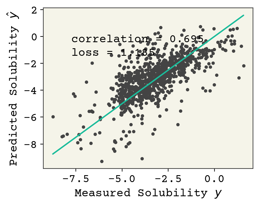
This performance is better than our simple linear model.

1.8. Exercises¶

Make a plot of the ReLU function. Prove it is non-linear
Try increasing the number of layers in the neural network. Discuss what you see in context of the bias-variance trade off
Show that a neural network would be equivalent to linear regression if \(\sigma(\cdot)\) was the identity function
What are the advantages and disadvantages of using deep learning instead of non-linear regression for fitting data? When might you choose non-linear regression over deep learning?

1.9. Chapter Summary¶

Deep learning is a category of machine learning that utilizes neural networks for classification and regression of data.
Neural networks are a series of operations with matrices of adjustable parameters.
A neural network transforms input features into a new set of features that can be subsequently used for regression or classification.
The most common layer is the dense layer. Each input element affects each output element. It is defined by the desired output feature shape and the activation function.
With enough layers or wide enough hidden layers, neural networks can approximate unknown functions.
Hidden layers are called such because we do not observe the output from one.
Using libraries such as TensorFlow, it becomes easy to split data into training and testing, but also to build layers in the neural network.
Building a neural network allows us to predict various properties of molecules, such as solubility.

Deep Learning for Molecules and Materials